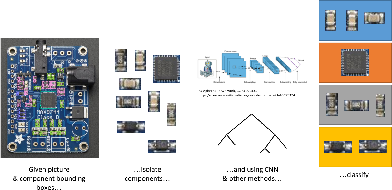
Visual analysis of the components on a printed circuit board (PCB) can provide additional security and quality assurance. For this reason, we decided to use existing computer vision techniques to classify PCB components by type (resistor, capacitor, etc.), achieving around 80% accuracy with the methodologies we tried.

Introduction

Recent events in the field of hardware security, whether true or not, have shined light on the issue of ensuring hardware security in a world where supply chains are not necessarily secure. In that light, ensuring that the components on a PCB are only those that are supposed to be there can improve security guarantees and, more prosaically, be useful for quality-assurance purposes. For this reason, we investigated visual classification of the components on PCBs using photographs taken with standard cameras using off-the-shelf computer vision products. Related work in this area includes defect analysis [1] and identification of specific PCBs for recycling purposes [2]. Such work extends back to at least the 90s as well [3].

Methodology

Dataset Generation

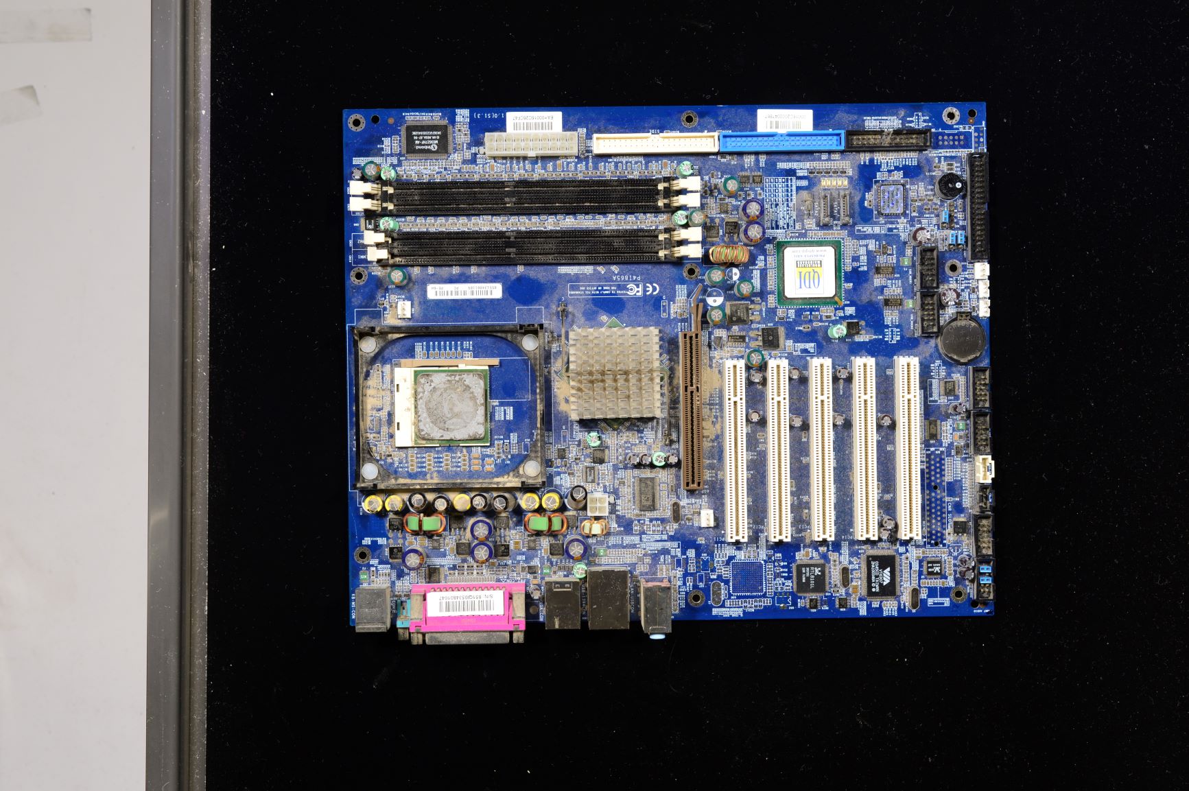
Before we could perform any form of object classification, we needed to find or generate a dataset of PCB components. We first searched for existing datasets. The only candidate we found in our search was the PCB DSLR Dataset from the Computer Vision Lab at TU Wien. This dataset consists of 748 high-resolution images of PCBs from a recycling facility, as well as segmentation information and bounding boxes. The authors’ stated intent for this dataset is that it be used to “facilitate research on computer-vision-based Printed Circuit Board (PCB) analysis, with a focus on recycling-related applications.”

Unfortunately, we decided after some review that this would not suffice for our purposes for a number of reasons.

• First, the dataset only contains segmentation information and bounding boxes for large integrated circuits (ICs), such as embedded processors and memory controllers. We sought to identify a wider variety of components.
• Next, dust and debris obscure many of the components on the PCBs in these images, a result of authors’ use of PCBs from a recycling center. This complicated our efforts to add our own segmentation information to the images.
• Furthermore, the large size of each image (4928x3280 pixels), meant it would be difficult to supplement the included labels with our own in a timely fashion.
• Finally, without detailed information about the design of the PCBs, we realized that we would not be able to generate sufficiently accurate annotations on our own.

Faced with these challenges, and with no other strong candidate datasets, we decided our best course of action involved generating our own dataset. We identified three criteria that needed to be met for our purposes:

• First, the PCBs in the images needed to contain a variety of components, including resistors, capacitors, diodes, inductors, LEDs, and ICs, but not in such quantities that hand-labeling them required an unreasonable amount of time.
• Next, each PCB needed to be clear of artifacts, whether visual (e.g., blurriness) or physical (e.g., dust).
• Finally, we needed access to a detailed listing of the components on each PCB, including their locations on the board, to allow accurate labeling of the ground truths for each image.

The third criterion in particular was a source of difficulty for us until we settled on the use of open-source hardware – hardware designs that include all of the necessary design files (e.g., EAGLE source files). As a result, we decided on constructing a database using images of products from Adafruit Industries, an open-source hardware company known for its support of electronic hobbyists. Adafruit provides the EAGLE source files for most of its internally-designed PCBs, allowing us to hand-label images of these PCBs with a high degree of accuracy.

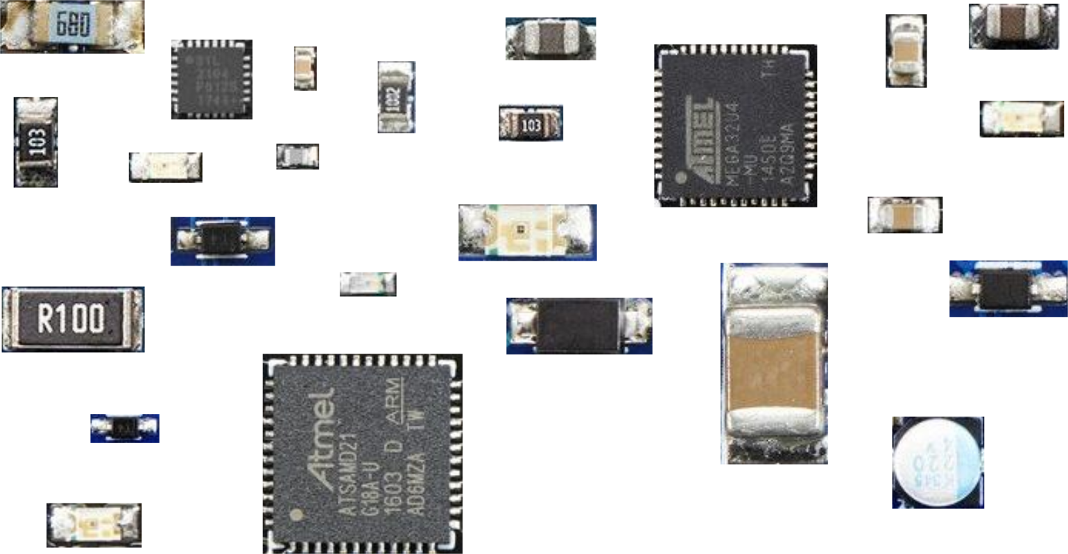
We identified six components for classification: resistors (R), capacitors (C), inductors (H), diodes (D), LEDs (L), and integrated circuits (ICs). For each image in our dataset, we used MATLAB’s Image Labeler tool to outline these components. The corresponding EAGLE PCB layout files served as our reference. From the resulting groundTruth objects, we extracted bounding boxes and cropped each image to generate our actual dataset of component images iand labels. Examples of the resulting images are shown below:

Object Classification

With our dataset generated, we moved onto the object classification problem. After researching the various methods available, we settled on testing two different approaches and comparing the accuracies. The first approach generated color histograms for each image and trained a variety of supervised classifiers using MATLAB’s Classification Learner tool. Specifically, this tool trains and scores the following types of learners in parallel:

• Decision Trees – data features used in a trained tree search to classify
• Support Vector Machines – data separated by hyperplanes based on similarity
• Nearest-neighbor Classifiers – using nearest-neighbor voting to determine similarity

The second approach used a convolutional neural network (CNN) implemented with MatConvNet [4]. Deep neural networks such as CNNs have wide applications to many fields of research, computer vision included, and seemed a suitable choice for this project due to their current popularity in the CV community.

The CNN used was a simple one, consisting of three convolutional layers separated by max-pooling layers and terminated by a soft-max-loss layer (for classification).

Results

For our dataset, we downloaded images and EAGLE source files for 25 different PCBs from Adafruit Industries (see above). Our final dataset contains 456 images of components. The image files and groundTruth objects can be found here; note that the name of each file corresponds to the product number at Adafruit.

Color histogram and Supervised Classifiers

We computed color histograms for each component by taking a histogram of each color channel (RGB). We used 10 bins for each color. As the number of pixels in each component image varies, we then normalized the histograms for each channel such that the sum of the 10-bin vector equals 1. Together, these gave us a feature vector 30 elements long.

We used these feature vectors to train a variety of different classifiers using MATLAB’s Classification Learner tool. The tool was set to automatically perform 5-fold cross-validation. The accuracies – that is, the percentage of correctly-classified components in the test set, averaged across all 5 folds – of the various classifiers are shown below:

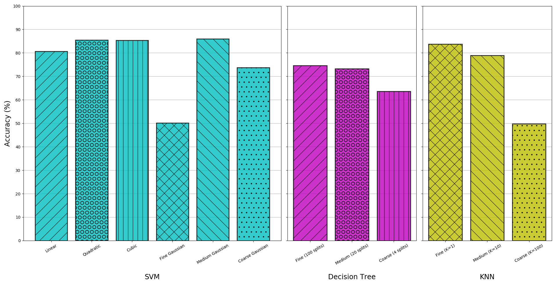
Overall, support vector machines provide the highest classification accuracy – the quadratic, cubic, and medium Gaussian kernels all perform about equally well with ~86% accuracies. The fine KNN classifier (K=1) also performed about as well as these three SVM models. Across the board, however, the finer the model’s granularity, the less effective it was; this suggests a need for a larger or more descriptive feature set.

Convolutional Neural Network

The figure below shows training of the CNN used over 75 epochs. We used four fifths of the component images, all resized to 32x32 and normalized on color values, for the training set and the remaining fifth as the validation set; in other words, this was one fold of a five-fold cross-validation. We chose 75 epochs as going beyond that seemed to result in overfitting on the training data (the objective function value for the validation set began increasing past that point as well as, to a lesser extent, the top-1 error).

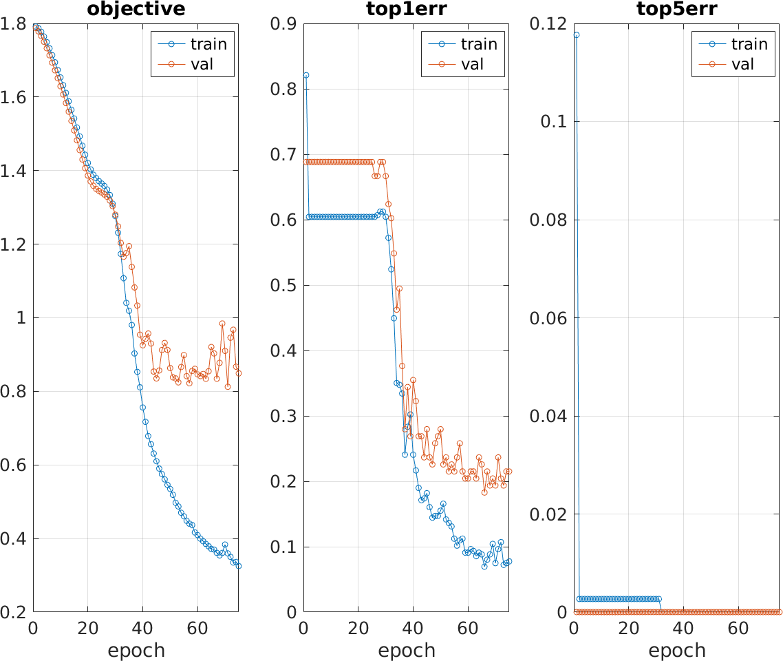
With full five-fold cross-validation, we obtained an average classification accuracy of 83.2% for the above-described CNN model.

Conclusion

Our achievement of around 80% accuracy with the classification methodologies we used illustrates that relying on proven tools and algorithms for PCB analysis is a viable route. Whether for purposes of security or simply quality assurance, companies and other organizations do not have to spend large amounts of money or large amounts of time to achieve product introspection via computer vision.

Further work on the CNN, perhaps using a deeper network or one with more data available, could improve accuracy beyond the level that we obtained with that approach. More fine-tuning of the non-neural-network approaches would also be useful; while color was indeed a significant factor, perhaps the primary factor, in distinguishing components, additional work using spatial features could improve accuracy. For all methods we attempted, we did not try masking the components with anything other than rectangular bounding boxes, so the background colors around the components may or may not have been factors in the accuracies of the methods used. Pursuing automatic extraction of components would also be a useful future contribution; our current manual approach is not scalable to large data sets. Higher-resolution images may also be useful for improved accuracy as they would provide additional per-component data points for the classification.

References

1. Bhardwaj, Sharat Chandra. “Machine vision algorithm for PCB parameters inspection.” In National Conference on Future Aspects of Artificial intelligence in Industrial Automation (NCFAAIIA 2012), Proceedings published by International Journal of Computer Applications®(IJCA), no. 2, pp. 20-24. 2012.
2. Pramerdorfer C., Kampel M. “PCB Recognition Using Local Features for Recycling Purposes”, Proc. 10th International Conference on Computer Vision Theory and Applications, pp. 71-78, Berlin, Germany, March 2015.
3. Moganti, Madhav, Fikret Ercal, Cihan H. Dagli, and Shou Tsunekawa. “Automatic PCB inspection algorithms: a survey.” Computer Vision and Image Understanding 63, no. 2 (1996): 287-313.
4. Vedaldi, Andrea, and Karel Lenc. “MatConvNet: Convolutional neural networks for Matlab.” In Proceedings of the 23rd ACM international conference on Multimedia, pp. 689-692. ACM, 2015.